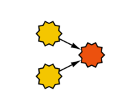The perceptron is the most basic form of an artificial neural network. In its simplest variant, it consists of a single neuron with one output and multiple inputs. Each input is associated with a connection weight, and the output is associated with an activation function. In the simplest case, the output consists of the value of the activation function for the weighted sum of the inputs. Learning a perceptron involves adjusting the weights of each neuron using a training dataset and the delta rule. A perceptron with *n* inputs separates the input space with an *(n−1)*-dimensional hyperplane. This illustrates the limitation of a perceptron’s capabilities. For example, the XOR function cannot be learned by a perceptron. The perceptron was introduced by Frank Rosenblatt in 1958.

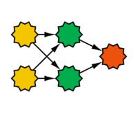Feedforward networks are an extension of the perceptron. In addition to the output layer, they also have a hidden layer, which is located between the input and output layers. The output of this hidden layer is invisible outside the network. A characteristic feature of feedforward networks is that there is a connection between each pair of nodes in adjacent layers, and the activation flow occurs only from input to output. Feedforward networks can overcome the limitations of the perceptron, allowing them to learn functions such as the XOR function. To train feedforward networks, backpropagation is used, which is a generalization of the delta rule. In this process, an error function is defined, such as the squared error between the desired and actual output. The goal is to find a minimum for this error function, though often only a local minimum is found. Weight adjustments are then made in the opposite direction of the gradient increase of the error function.

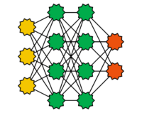This refers to feedforward networks with more than one hidden layer, which are used in what is called deep learning. As the number of layers and neurons increases, so does the computational effort required to train deep feedforward networks. Therefore, many-core systems, graphics processors (GPUs), or tensor processing units (TPUs) are often used. In recent years, deep feedforward networks have achieved spectacular successes, such as in pattern recognition. Freely available software libraries for deep feedforward networks, such as TensorFlow or PyTorch, have led to their widespread adoption in recent years. When training deep feedforward networks, the layers are often considered sequentially.

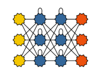Recurrent neural networks (also called feedback neural networks) differ from feedforward networks by having connections from neurons in one layer to neurons in the same or a previous layer. This recurrence acts as short-term memory. Recurrent neural networks are well-suited for learning time series, such as for classifying temporal sequences or for time series forecasting. Training recurrent neural networks is more complex than training feedforward networks. The feedback loops complicate the direct application of backpropagation. These feedback loops are often addressed by unfolding the network over time between two or even several input data sets.

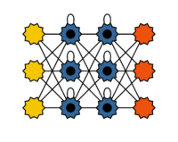
Long Short-Term Memory (LSTM) networks are a special type of recurrent neural network designed to learn long-term dependencies. In this case, the short-term memory of recurrent neural networks is extended to a long short-term memory. The success of LSTMs is largely due to training with large datasets and the use of powerful hardware. Neural networks with many layers, in particular, benefit from LSTMs. The distinctive feature of LSTM networks is the structure of the memory cell, which consists of so-called gates. These gates control which values flow into the cell, remain in the cell or are forgotten, and which values are passed on. LSTMs are used in applications like speech recognition on smartphones.

Autoenc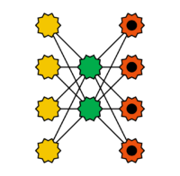oders are feedforward networks used for learning encodings. In addition to the input layer, they consist of at least two layers: an input layer, some significantly smaller hidden layers that form the codings, and an output layer, where each neuron has the same meaning as the corresponding one in the input layer. Autoencoders enforce the discovery of the best representation of the input. If the number of hidden neurons is smaller than the number of inputs, this leads to dimensionality reduction. After training, the input layer to the first hidden layer acts as the encoder, while the last hidden layer acts as the decoder. Autoencoders belong to the group of unsupervised learning methods. Special types of autoencoders include stacked autoencoders and denoising (stacked) autoencoders. In stacked autoencoders, after training the first two layers, two more are added between them and trained. This process can be repeated by adding and training additional layers between the new ones. Denoising autoencoders are trained to compute clean outputs from slightly corrupted inputs.

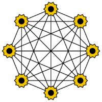A Hopfield network is a special type of artificial neural network. It consists of only a single layer, which functions simultaneously as both the input and output layer. Each neuron is connected to every other neuron, except itself. The neurons can take on values of −1 and 1. Hopfield networks are often used as associative memory, allowing the recognition of stored patterns. During the training phase, incomplete or noisy patterns are used. This type of network was introduced by John Hopfield in 1982.

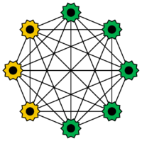Boltzmann machines are a special type of Hopfield network. Some of the neurons serve as input neurons, while the rest form a hidden layer. The neurons can only take values of 0 or 1, but they behave stochastically. Input neurons become output neurons once all hidden neurons have changed their state. The training of Boltzmann machines is often done using simulated annealing. They are named after the Boltzmann distribution in thermodynamics. Boltzmann machines were developed in 1985 by Geoffrey Hinton and Terrence J. Sejnowski.

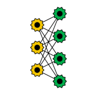
Without restrictions on the connections, Boltzmann machines are very difficult to train. If the connections between the neurons are restricted, the learning process is greatly simplified. Connections between the input and hidden neurons are eliminated. Restricted Boltzmann Machines are used in many practical applications, such as in speech processing. Training is performed using backpropagation, similar to feedforward networks. Restricted Boltzmann Machines were introduced by Smolensky in 1986.

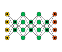Deep Belief Networks (DBNs) are coupled simple networks, such as Boltzmann machines or autoencoders. The idea is that each individual layer recognizes a feature of the input and passes its output to the next layer. This allows the input to be progressively filtered. Training occurs in a greedy fashion: the layers are trained sequentially, one at a time. Deep Belief Networks play a significant role in applications such as image and video recognition.

Kohonen networks are feedforward networks that consist of an input layer and only one additional layer, known as the Kohonen layer. The fundamental idea is to create a structure of interconnected processing units (neurons). The weights of the connections are adjusted using an unsupervised learning rule. They are used for classification and clustering tasks. The name originates from the Finnish engineer Teuvo Kohonen, who introduced this concept in 1982.

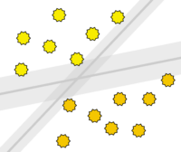Support Vector Machines (SVMs) refer to a statistical approach for classifying objects into two categories. They are used for both linear and non-linear classification. The classification aims to maintain the widest possible margin free of objects around the class boundaries. One advantage of this method is that it can work well with relatively few training samples while still achieving high accuracy. Generally, the performance of the method tends to degrade as the training data become noisier.